Scroll and read through your original 119-page lecture notes directly below, or reference them alongside each interactive concept in the study guide.
PART 01CORE FOUNDATION • 3M / 6M
Transport Layer Services & Principles
PDF Pages: 1 – 6
💡 What is the Transport Layer?
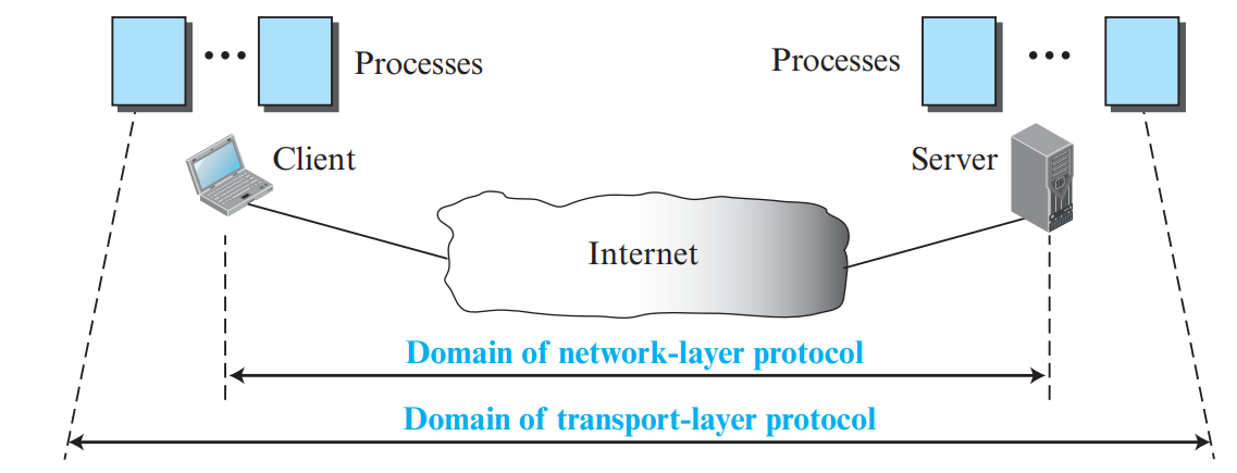
While the Network Layer provides host-to-host communication (delivering datagrams between computers), the Transport Layer provides process-to-process logical communication (delivering messages between specific running programs on those computers).
1. Addressing: Port Numbers & Sockets
Operating systems run dozens of application processes simultaneously. To route data to the correct application, the transport layer uses Port Numbers (16-bit integers ranging from 0 to 65535):
Port Range
Category Name
Usage & Authority
0 – 1023
Well-Known / Standard Ports
Assigned and controlled by IANA for standard universal server services (HTTP = 80, HTTPS = 443, FTP = 20/21, SMTP = 25, DNS = 53).
1024 – 49151
Registered Ports
Not assigned automatically; organizations can register them with IANA to avoid conflicts.
49152 – 65535
Dynamic / Private / Ephemeral
Assigned dynamically by the local OS to client processes for the duration of a session.
Figure 1.1: Process-to-Process Communication via Port Addressing (Page 1)
🔑 Core Concept: Socket Address
A Socket Address is the unique combination of an IP Address (identifying the host machine on the network) and a Port Number (identifying the specific application process within that host):
A full-duplex communication channel is uniquely identified globally by a Socket Pair (5-tuple: Source IP, Source Port, Destination IP, Destination Port, Transport Protocol).
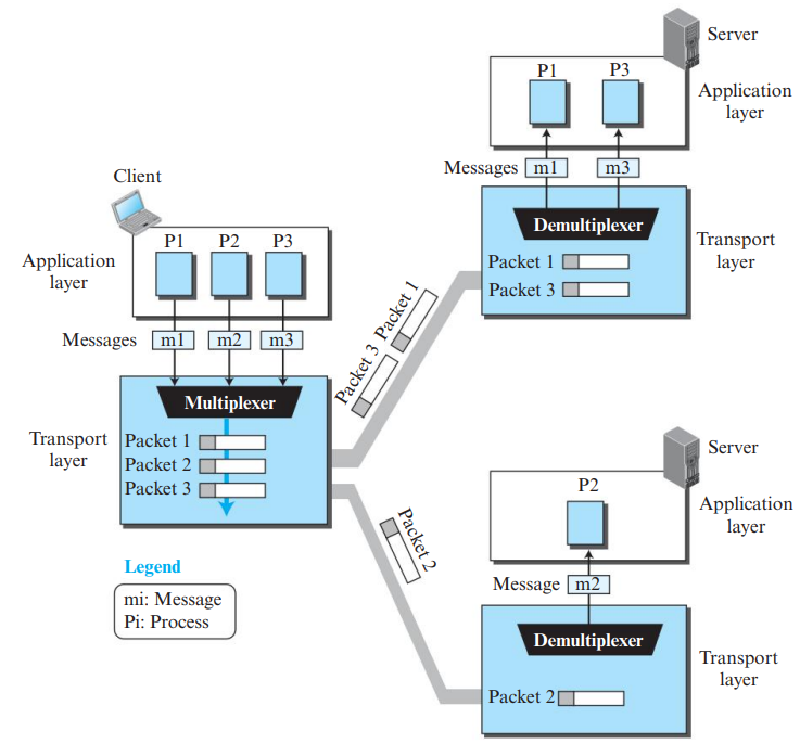
2. Multiplexing and Demultiplexing
Multiplexing (Sender): Transport layer collects data chunks from multiple application sockets, adds transport headers (including source and destination port numbers), and passes segments down to the Network layer.
Demultiplexing (Receiver): Transport layer inspects the destination port number in the received segment and directs the payload to the corresponding application socket.
Connectionless (UDP) Demultiplexing: Uses only 2-tuple: (Destination IP, Destination Port).
Transport Layer Protocols: Stop-and-Wait, Go-Back-N & Selective Repeat
PDF Pages: 7 – 18
💡 Evolution of Transport Protocols
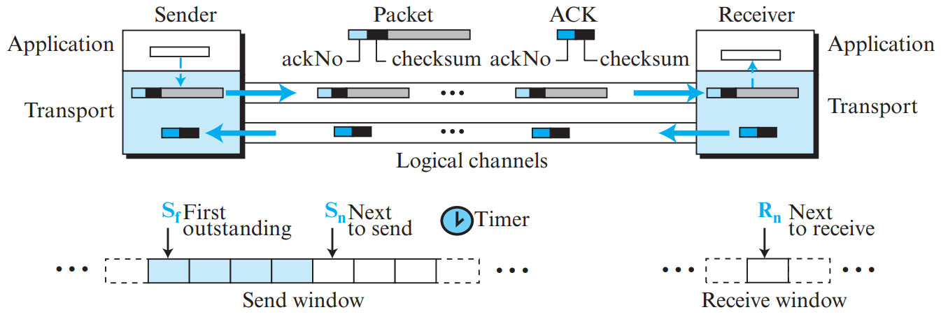
To achieve reliable transmission over an unreliable underlying network, protocols evolved from simple Stop-and-Wait to sophisticated sliding-window pipelined protocols: Go-Back-N (GBN) and Selective Repeat (SR).
1. Stop-and-Wait Protocol
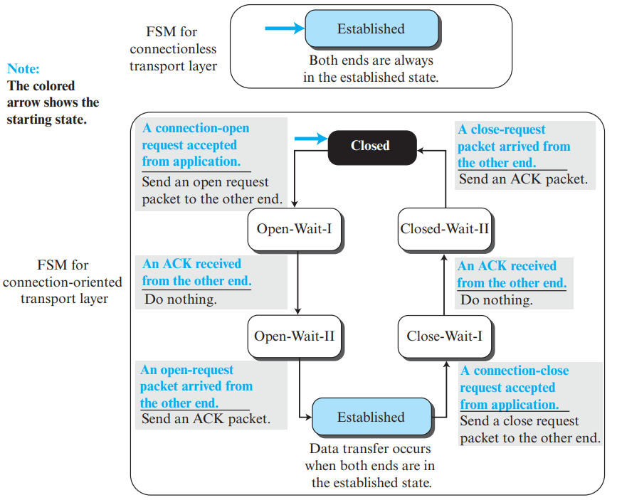
Sender transmits one packet and stops. It waits until an acknowledgment (ACK) is received before sending the next packet. Uses 1-bit sequence numbers (0 and 1).
Lost Packet: Sender's retransmission timer expires; sender resends the same packet.
Lost ACK: Sender times out and resends packet. Receiver detects duplicate via sequence number, discards duplicate, and re-sends ACK.
Efficiency: Very poor utilization on high-bandwidth-delay product links (\(\text{Efficiency} = \frac{T_t}{T_t + 2T_p}\)).
📐 High-Frequency KTU Question: Why Must \(W_s < 2^m\) in Go-Back-N?
If window size \(W_s = 2^m\), suppose the sender sends packets \(0\) to \(2^m - 1\). All packets arrive safely, but all ACKs are lost. The sender times out and re-sends packet \(0\). However, the receiver's window has already advanced to the next cycle and is expecting packet \(0\) of the *next* round! The receiver cannot distinguish between a retransmitted duplicate and a brand-new packet. Hence, \(W_s \le 2^m - 1\).
PART 03CORE PROTOCOL • 3M / 5M
User Datagram Protocol (UDP)
PDF Pages: 19 – 22
💡 What is UDP?
UDP is an extremely lightweight, connectionless, unreliable transport protocol. It provides minimal transport service beyond IP: port addressing and optional error detection via checksum.
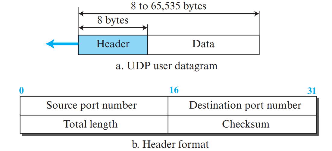
1. UDP Header Format (8 Bytes Fixed)
The UDP header is strictly 8 bytes (64 bits) long, divided into four 16-bit fields:
Figure 3.1: 8-Byte Fixed UDP Header Format (Page 20)
Header Field
Length
Description & Purpose
Source Port
16 bits
Port number of the sending process (optional; set to 0 if no reply is expected).
Destination Port
16 bits
Port number of the receiving process (mandatory for delivery).
Total Length
16 bits
Total length of UDP user datagram in bytes (\(\text{Header} + \text{Data}\)). Minimum value = 8.
Checksum
16 bits
Optional in IPv4 (all 0s if unused), mandatory in IPv6. Covers UDP pseudo-header, header, and data.
📐 High-Frequency KTU Numerical: Maximum UDP Payload Size
Since the IP Total Length field is 16 bits, the maximum size of an IP datagram is \(2^{16} - 1 = 65535\) bytes. Subtracting the minimum 20-byte IP header and the 8-byte UDP header:
To detect errors, UDP computes a 16-bit One's complement (1's complement) sum using Protocol 17. It includes a 12-byte Pseudo-Header borrowed from the IP layer (Source IP, Destination IP, All 0s, Protocol = 17, UDP Length) to verify that the datagram reached the correct destination host!
3. Why Choose UDP Over TCP? & UDP Datagram vs. TCP Segment
The transport PDU in UDP is formally known as a UDP Datagram (or User Datagram). Unlike TCP, UDP provides no connection setup, no flow control, and no retransmissions, leading to extremely low overhead:
No Connection Delay: Zero setup RTT latency; transmits data immediately (DNS, DHCP).
No Congestion Throttling: Transmits at real-time rate even during packet loss (VoIP, live video streaming, online gaming).
Small Header Overhead: Only 8 bytes compared to TCP's 20–60 bytes.
Multicasting & Broadcasting: Only UDP supports one-to-many communication; TCP is strictly point-to-point unicast.
PART 04VERY HIGH PRIORITY • 5M / 9M ESSAY
Transmission Control Protocol (TCP): Architecture & Connection
PDF Pages: 22 – 31
💡 What is TCP?
TCP is a connection-oriented, reliable, byte-stream transport protocol. It provides full-duplex communication and creates the illusion of an unbroken logical "tube" carrying data between two processes.
TCP provides a Stream-oriented (byte-stream) service. Applications write a continuous sequence of bytes into the TCP socket, and TCP packages these bytes into segments. Each byte is numbered using an Initial Sequence Number (ISN).
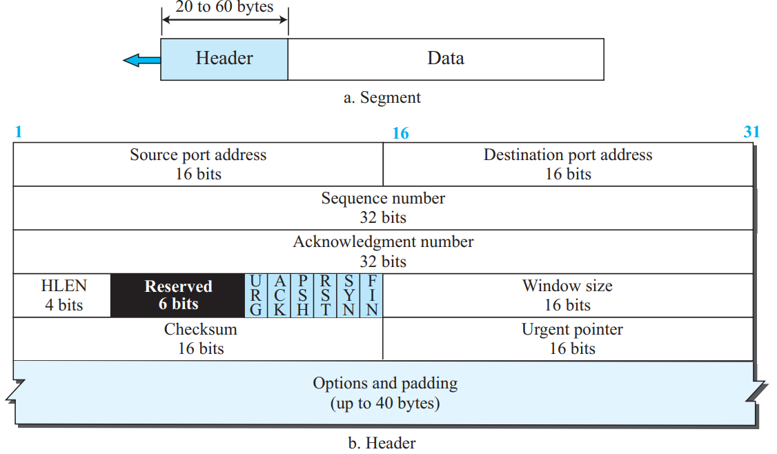
1. TCP Segment Format (20 to 60 Bytes)
The TCP header has a minimum length of 20 bytes and a maximum of 60 bytes (depending on optional fields):
Figure 4.1: TCP Segment Header Format (Page 25)
Field Name
Bit Width
Technical Description
Source Port / Dest Port
16 bits each
Identifies sending and receiving application process.
Sequence Number
32 bits
Byte sequence number of the first data byte in this segment.
Acknowledgment Number
32 bits
Cumulative ACK: contains the next expected byte number from sender. Valid if ACK flag = 1.
HLEN (Header Length / Data offset)
4 bits
Specifies number of 4-byte words in header. Range 5 to 15 (i.e., \(5 \times 4 = 20\) to \(15 \times 4 = 60\) bytes).
Reserved
6 bits
Reserved for future use.
Control Flags (URG, ACK, PSH, RST, SYN, FIN)
6 bits (1 bit each)
URG: Urgent pointer valid. ACK: Acknowledgment number valid. PSH: Push data immediately to application. RST: Reset/abort connection. SYN: Synchronize sequence numbers during connection establishment. FIN: Terminate connection; no more data from sender.
Window Size (rwnd)
16 bits
Receiver's advertised buffer space in bytes for flow control (max 65,535 bytes without scaling).
Checksum
16 bits
Mandatory error detection over pseudo-header, TCP header, and data.
Urgent Pointer
16 bits
Offset added to sequence number pointing to end of urgent data (if URG = 1).
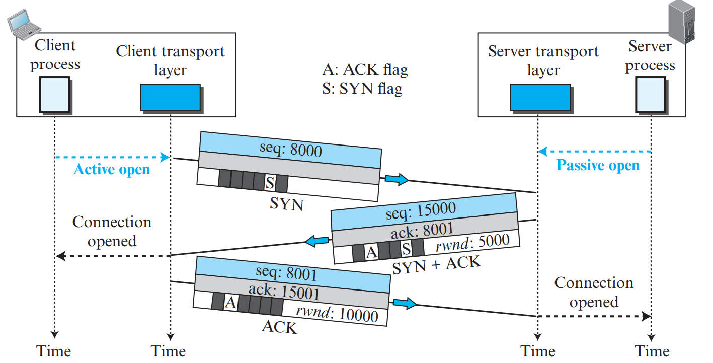
Step 1 (SYN segment from Client to Server): Client chooses an Initial Sequence Number (\(ISN_c = x\)), sets flag SYN = 1. Consumes 1 sequence number. Carries no data.
Step 2 (SYN + ACK segment from Server to Client): Server allocates buffers, chooses its own sequence number (\(ISN_s = y\)), sets SYN = 1 and ACK = 1, and confirms client sequence by setting \(\text{ACK Number} = x + 1\). Consumes 1 sequence number.
Step 3 (ACK segment from Client to Server): Client acknowledges server: sets ACK = 1, \(\text{Seq} = x + 1\), and \(\text{ACK Number} = y + 1\). May carry first application data bytes!
Either party can close the connection. Since TCP is full-duplex, each direction closes independently:
Client sends FIN (\(\text{Seq} = u\)). Server replies with ACK (\(u + 1\)). (Client-to-server direction is closed).
Server continues sending remaining data. When finished, Server sends its own FIN (\(\text{Seq} = v\)).
Client replies with ACK (\(v + 1\)) and enters TIME-WAIT state for \(2 \times \text{MSL}\) (Maximum Segment Lifetime, typically 2 minutes) to ensure server receives final ACK.
PART 05VERY HIGH PRIORITY • 5M / 9M ESSAY
TCP Flow Control, Error Control & Congestion Control
PDF Pages: 32 – 54
💡 The Triad of TCP Reliability
TCP coordinates three distinct control loops: Flow Control (protects receiver buffer), Error Control (recovers lost data), and Congestion Control (protects intermediate network routers).
1. TCP Flow Control & Sliding Window
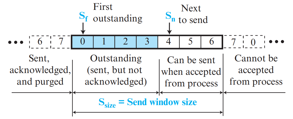
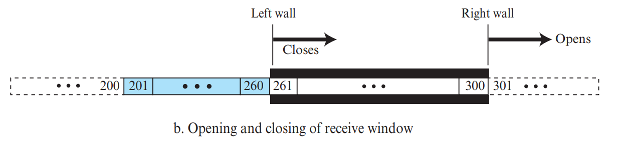
TCP uses a byte-oriented sliding window with dynamic Credit Allocation: the receiver grants the sender credit (\(rwnd\)) to transmit up to that many bytes before stopping. sliding window. The receiver advertises its available buffer space in the Window Size (rwnd) field of every ACK. The sender's usable window cannot exceed \(rwnd\).
Figure 5.1: Allocated Buffer & Sliding Window at Sender and Receiver (Page 33)
Silly Window Syndrome & Solutions
Occurs when data is generated in tiny chunks (e.g., 1 byte from a terminal), resulting in a massive 41-byte packet (20B IP + 20B TCP + 1B data) with 97.5% overhead!
Nagle's Algorithm (Sender-Side): Sender sends the first byte immediately. All subsequent small writes are buffered until either an entire Maximum Segment Size (MSS) is accumulated, or the previous ACK is received.
Clark's Solution (Receiver-Side): Receiver prevents advertising tiny window updates. It advertises rwnd = 0 until it can open a window of at least one full MSS or half of its total buffer.
2. TCP Congestion Control: AIMD, Slow Start & Fast Recovery
The effective transmission window is the minimum of receiver window and congestion window: \(\text{Send Window} = \min(rwnd, cwnd)\).
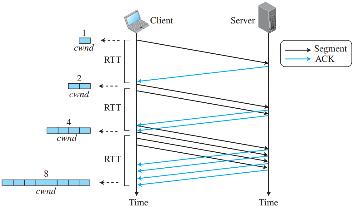
Starts at \(cwnd = 1 \text{ MSS}\). Doubles exponentially every RTT (\(1 \rightarrow 2 \rightarrow 4 \rightarrow 8 \dots\)) for each ACK received.
Continues until \(cwnd\) reaches the Slow Start Threshold (\(ssthresh\)).
2. Congestion Avoidance
Increases linearly by \(1 \text{ MSS}\) per RTT (Additive Increase).
Continues until packet loss/timeout occurs.
3. Congestion Detection
• Timeout: Severe congestion. Set \(ssthresh = cwnd / 2\), reset \(cwnd = 1\), restart Slow Start.
• 3 Duplicate ACKs: Mild congestion (TCP Reno). Fast Retransmit missing packet; set \(ssthresh = cwnd / 2\), set \(cwnd = ssthresh + 3\), enter Fast Recovery!
Avoids resetting to 1 MSS during isolated packet losses.
3. TCP Timers (PDF Pages 48 – 52)
Retransmission Timer (RTO): Tracks unacknowledged segments; retransmits upon expiration. Dynamically calculated using Smoothed RTT (SRTT) and Round-Trip Time Variation (RTTVAR).
Persistence Timer: Prevents deadlock when receiver advertises rwnd = 0 and the subsequent window update ACK is lost. Periodically sends 1-byte probe packets to prompt receiver for updated window size.
Keepalive Timer: Detects dead clients in idle connections (typically 2 hours).
TIME-WAIT Timer: Enforces a \(2 \times \text{MSL}\) delay before closing to ensure the final ACK arrives and prevents old duplicate packets from interfering with new connections.
Silly Window Syndrome occurs when data is exchanged in tiny increments (e.g. 1 byte of application payload wrapped in 40 bytes of TCP/IP headers), causing extreme bandwidth waste:
Sender-side Syndrome & Nagle's Algorithm (Nagle algorithm): Solves the problem where applications produce data 1 byte at a time (e.g., Telnet keystrokes).
Nagle's Rule: The sender transmits the first piece of data immediately. While waiting for the acknowledgment (ACK), the sender accumulates all subsequent application data in its buffer. It sends the next segment ONLY when either:
A full Maximum Segment Size (MSS) worth of data has been collected, OR
The pending ACK for previous data arrives.
Receiver-side Syndrome & Clark's Solution: Occurs when the receiving application consumes data 1 byte at a time, advertising 1-byte window updates. Clark's solution prevents the receiver from advertising small window increases: the receiver waits until either a full MSS of buffer space is free or at least 50% of the buffer is empty before sending a window update.
5. Round-Trip Time (RTT) Estimation & Karn's Algorithm (Karn algorithm)
TCP calculates its Retransmission Timeout (RTO) using measured Round-Trip Times (RTT). However, when a packet is retransmitted and an ACK arrives, an ambiguity arises: Does the ACK correspond to the original packet or the retransmitted packet?
📐 Karn's Algorithm Rules
Karn's algorithm resolves this measurement ambiguity with two strict principles:
Rule 1: Do not measure or update the RTT estimate using ACKs for segments that have been retransmitted.
Rule 2 (Timer Backoff): Whenever a retransmission occurs, double the current RTO value using exponential backoff:
\[\text{RTO}_{\text{new}} = 2 \times \text{RTO}_{\text{old}}\]
Continue doubling on successive retransmissions until a segment is transmitted and acknowledged without any retransmission.
PART 06VERY HIGH PRIORITY • 5M / 9M ESSAY
Network Layer Introduction & IPv4 Protocol
PDF Pages: 55 – 66
💡 What is the Network Layer?
The Network Layer provides host-to-host delivery of packets across multiple intermediate network hops. It handles packetizing, routing, forwarding, and logical addressing.
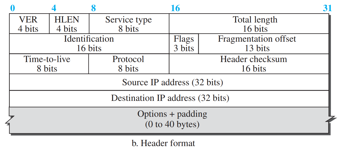
1. IPv4 Datagram Header Format (20 to 60 Bytes)
Figure 6.1: IPv4 Datagram Header Format (Page 57)
Header Field
Bits
Technical Function & Examination Role
VER (Version)
4 bits
Defines IP version (always 4 for IPv4, binary 0100).
HLEN (Header Length / Data offset)
4 bits
Length of header in 4-byte multiples. Minimum value is 5 (\(5 \times 4 = 20\) bytes).
Type of Service (DS / ECN)
8 bits
Specifies packet priority / Quality of Service (Differentiated Services).
Total Length
16 bits
Total length of datagram (\(\text{Header} + \text{Data}\)). Max = 65,535 bytes.
Identification
16 bits
Unique ID assigned by sender to identify all fragments of the same original datagram.
Flags (DF & MF)
3 bits
Bit 0: Reserved (0).
Bit 1 (DF - Don't Fragment): If 1, router cannot fragment; if packet exceeds MTU, router drops it and sends ICMP error.
Bit 2 (MF - More Fragments): 1 means more fragments follow; 0 means this is the last fragment.
Fragment Offset
13 bits
Relative position of data fragment in original datagram, measured in 8-byte units (\(\text{Offset} = \text{Byte Position} / 8\)).
Time to Live (TTL)
8 bits
Hop limit counter. Decremented by 1 at each router. When \(\text{TTL} = 0\), datagram is discarded to prevent infinite routing loops.
1's complement checksum covering only the header (recalculated at every router due to TTL decrement!).
Source / Destination IP
32 bits each
Globally unique logical addresses of sender and recipient.
2. IPv4 Fragmentation & MTU Calculation
Each physical link technology has a Maximum Transmission Unit (MTU) (e.g., Ethernet MTU = 1500 bytes). When a datagram is larger than the outgoing link's MTU, routers fragment it.
📐 High-Frequency KTU Numerical: IP Datagram Fragmentation
Problem: An IP datagram with total length 4000 bytes (including a 20-byte header) must pass through a link with an MTU of 1500 bytes. Find the number of fragments, total length, fragment offset, and MF flag for each fragment.
Solution:
Total data = \(4000 - 20 = 3980\) bytes.
Maximum data per fragment = \(1500 - 20 = 1480\) bytes (must be a multiple of 8; \(1480 / 8 = 185\), perfectly divisible!).
Fragment 1:
Data bytes 0 to 1479 (1480 bytes).
Total length = \(1480 + 20 = \mathbf{1500 \text{ bytes}}\).
Fragment offset = \(0 / 8 = \mathbf{0}\).
MF flag = \(\mathbf{1}\) (more fragments follow).
Fragment 2:
Data bytes 1480 to 2959 (1480 bytes).
Total length = \(1480 + 20 = \mathbf{1500 \text{ bytes}}\).
Fragment offset = \(1480 / 8 = \mathbf{185}\).
MF flag = \(\mathbf{1}\).
Fragment 3:
Remaining data = \(3980 - (1480 \times 2) = 1020\) bytes.
Total length = \(1020 + 20 = \mathbf{1040 \text{ bytes}}\).
Fragment offset = \(2960 / 8 = \mathbf{370}\).
MF flag = \(\mathbf{0}\) (last fragment!).
🌐 Special IPv4 Address Ranges
Loopback Address (127.0.0.1 or 127.0.0.0/8): Used for local host testing; datagrams never leave the local system.
Private IP Ranges (RFC 1918): Reserved for private local networks, not routable on the public Internet:
Class A: 10.0.0.0/8 (10.0.0.0 to 10.255.255.255)
Class B: 172.16.0.0/12 (172.16.0.0 to 172.31.255.255)
Class C: 192.168.0.0/16 (192.168.0.0 to 192.168.255.255)
Limited Broadcast Address (255.255.255.255): Broadcasts to all hosts on the local physical subnet; blocked by routers.
PART 07VERY HIGH PRIORITY • 5M / 9M ESSAY
IPv4 Addressing: Classful, CIDR Subnetting & NAT
PDF Pages: 67 – 75
💡 What is an IP Address?
An IPv4 address is a 32-bit identifier that uniquely and universally defines the connection of a host or router to the Internet. Written in dotted-decimal notation (e.g., 192.168.1.1).
Classful addressing caused massive address waste. Today, the Internet uses Classless Inter-Domain Routing (CIDR). An address is written with a slash notation: address /n, where \(n\) is the prefix length (number of 1s in the mask).
📐 High-Frequency KTU Subnetting Numerical
Problem: A host has IP address 172.16.45.200/26. Find:
The subnet mask.
The network address and broadcast address.
The usable host address range and number of usable hosts.
5. Usable Host Range:
From first host (\(\text{Network} + 1\)) to last host (\(\text{Broadcast} - 1\)):
\(\mathbf{172.16.45.193 \text{ to } 172.16.45.254}\).
Number of usable hosts = \(2^6 - 2 = 64 - 2 = \mathbf{62 \text{ hosts}}\).
Figure 7.1: Address Aggregation and Subnetting at Router (Page 68)
🔍 Forwarding Table Lookup & Longest Prefix Match (LPM)
In classless addressing, routes in a router's Forwarding Table are organized by prefix lengths. When a packet arrives, the router may find multiple matching routing entries for the destination IP address.
Longest Prefix Match Rule: The router selects the routing table entry with the longest mask length (the most specific route with the highest number of 1s in the subnet mask). For example, a destination matching both 128.96.34.0/24 and 128.96.0.0/16 is routed via the /24 interface because it is more specific.
3. Network Address Translation (NAT) & NAPT
Allows thousands of devices on a private network to share a single public IP address when communicating on the Internet.
Private Address Ranges (RFC 1918):
10.0.0.0/8 (10.0.0.0 to 10.255.255.255)
172.16.0.0/12 (172.16.0.0 to 172.31.255.255)
192.168.0.0/16 (192.168.0.0 to 192.168.255.255)
NAPT (Network Address Port Translation): Router replaces (Private IP, Private Port) with (Public IP, Router Ephemeral Port) and tracks entries in a NAT translation table.
PART 08VERY HIGH PRIORITY • 5M / 9M ESSAY
Unicast Routing Protocols: Distance Vector, Link State & Path Vector
PDF Pages: 76 – 88
💡 Unicast Routing Overview
Routing is the process of selecting the optimal path across a network of interconnected routers. Routing protocols are broadly classified into Intra-Domain (Interior Gateway Protocols / IGP) and Inter-Domain (Exterior Gateway Protocols / EGP).
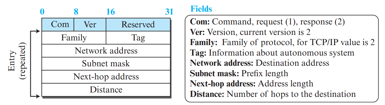
In RIP, the distance metric is defined by Hop count (each router traversed adds 1 hop). The maximum valid path is 15 hops; 16 hops indicates infinity (unreachable destination).
Each router maintains a vector (table) of minimum distances to all known destinations. Routers periodically share their entire routing vector with their direct immediate neighbors only.
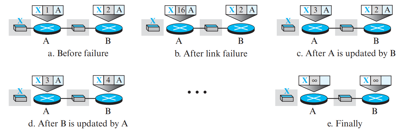
Occurs when a link fails. Because routers update based on second-hand information, a routing loop is created where distance to unreachable node increments slowly to infinity (\(\infty = 16\) in RIP).
Split Horizon: A router does not advertise a route back out the same interface from which it learned that route!
Poisoned Reverse: The router advertises the route back, but explicitly marks its cost as \(\infty\) ("poison"), instantly killing the loop.
⚠️ The Count-to-Infinity Problem & Poison Reverse
A classic instability in Distance Vector routing occurs when a link breaks. Two neighboring routers falsely inform each other of an alternate route, incrementing their distance metrics indefinitely until reaching infinity (16 in RIP):
Split Horizon: A router never advertises a route back out the same interface through which it learned that route.
Split Horizon with Poison Reverse: A router does advertise the route back out the same interface, but explicitly sets the metric to \(\infty\) (16), saying "You told me how to get there; do not try to reach it through me!" This immediately eliminates two-node routing loops.
2. Link State Routing (Dijkstra's Algorithm & OSPF)
Each router discovers its direct neighbors, packages their states into a Link State Advertisement (LSA), and floods it to every router in the entire network. Every router builds an identical Link State Database (LSDB) representing the complete network topology graph, and runs Dijkstra's Shortest Path Algorithm locally.
Figure 8.2: Link State Routing & OSPF Area Hierarchy (Page 85)
Comparison Parameter
Distance Vector (RIP)
Link State (OSPF)
Knowledge of Topology
Tells its neighbors about the entire world. Has only local view.
Tells the entire world about its local neighbors. Has full global map!
Algorithm Used
Distributed Bellman-Ford algorithm.
Dijkstra's shortest path algorithm.
Convergence Speed
Slow convergence; vulnerable to count-to-infinity.
Fast convergence; no routing loops.
Scalability & Hierarchy
Limited to max 15 hops.
Supports two-level hierarchical Areas (Backbone Area 0).
Inter-domain routing protocol used between Autonomous Systems (AS). Instead of just cost, BGP advertises the entire sequence of Autonomous Systems (the AS-PATH attribute) required to reach a destination prefix.
Loop Prevention: If a router sees its own Autonomous System number inside the received AS-PATH, it rejects the route immediately!
Policy Routing: Network administrators can enforce economic, political, and security policies when choosing transit paths.
🏛️ OSPF Hierarchical Architecture: Areas, ABR & ASBR
Backbone Area (Area 0): The core central area that connects all other secondary areas. All inter-area traffic must transit Area 0.
Area Border Router (ABR): A router with interfaces attached to multiple areas (at least one interface in Area 0). Summarizes and advertises routes between areas.
Autonomous System Boundary Router (ASBR): A router that interfaces with external networks or runs other routing protocols (like BGP or RIP), redistributing external routes into OSPF.
🌐 External BGP (eBGP) vs. Internal BGP (iBGP)
eBGP (External BGP): Used between border routers belonging to different Autonomous Systems to exchange reachability information and inter-AS policies.
iBGP (Internal BGP): Used to distribute the externally learned BGP routing information among all internal routers within the same Autonomous System.
PART 09EXAMINATION ESSAY • 5M / 9M
Multicast Routing Protocols: DVMRP, MOSPF & PIM
PDF Pages: 89 – 105
💡 What is Multicasting?
One-to-many communication where a sender transmits a single packet, and network routers replicate that packet only at branching points to reach all subscribed members of a Multicast Group (Class D IP: 224.0.0.0 to 239.255.255.255).
1. Unicast vs Multicast: Foundational Concepts
Network communication can be categorized based on the number and specificity of recipients:
Paradigm
Source
Destination
Bandwidth Efficiency
Key Protocols
Unicast
One host
One specific host
N separate streams for N receivers (wasteful for group video)
HTTP, SSH, FTP, TCP/UDP
Multicast
One host
A specific group of subscribed hosts
One stream replicated by routers only at branch points (optimal)
IGMP, DVMRP, MOSPF, PIM
Broadcast
One host
All hosts on the subnet
Sent to all nodes regardless of interest (causes broadcast storms)
ARP request, DHCP discover
Anycast
One host
Nearest of multiple identical servers
Routes to topologically closest server instance
DNS Root servers, CDNs
2. Multicast Routing Trees: Source-Based vs. Group-Shared
Feature
Source-Based Tree (Shortest Path Tree)
Group-Shared Tree (Core-Based Tree)
Tree Construction
A separate unique tree is constructed for every individual source in the multicast group (\(m\) sources \(\rightarrow m\) trees).
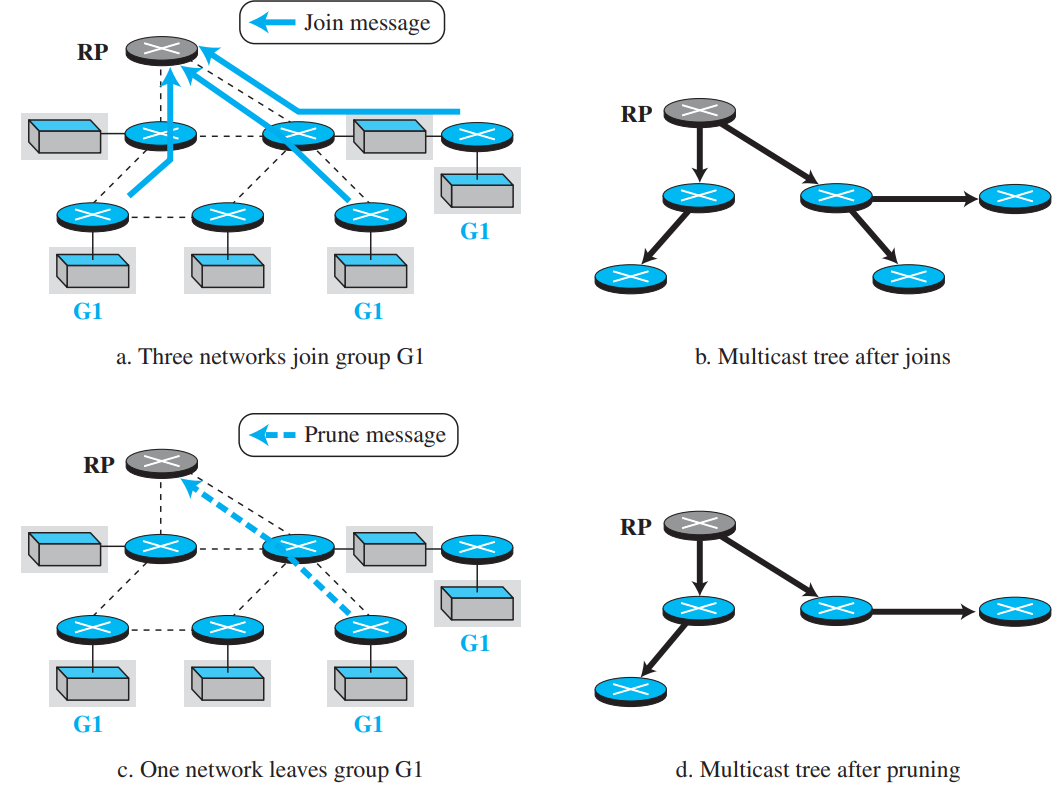
A single shared tree is constructed centered at a designated Rendezvous Point (RP) / Core Router.
Router Memory Overhead
High (\(O(S \times G)\) state in routers).
Low (\(O(G)\) state in routers).
Path Optimality
Optimal shortest path from each source to every receiver.
Sub-optimal (packets first route to core, causing "tromboning" delay).
Protocols
DVMRP, MOSPF, PIM-DM.
PIM-SM, CBT.
Figure 9.1: Group-Shared Tree with Rendezvous Point (RP) in PIM-SM (Page 102)
Reverse Path Forwarding (RPF): Accepts a packet only if it arrives on the interface used to reach the source. Prevents loops.
Reverse Path Multicasting (RPM): First floods network, then uses Prune messages to cut off non-member branches, and Graft messages when new members join.
MOSPF (Multicast OSPF): Source-based tree built on-demand using Dijkstra's algorithm over OSPF database.
PIM (Protocol Independent Multicast): Operates over any underlying unicast routing table.
PIM-DM (Dense Mode): Floods and prunes (for dense groups like LANs).
PIM-SM (Sparse Mode): Explicit join messages to a Rendezvous Point (RP) (for wide-area Internet).
PART 10VERY HIGH PRIORITY • 5M / 9M ESSAY
Next-Generation IP (IPv6) & Transition Strategies
PDF Pages: 106 – 112
💡 Why IPv6?
IPv4 has run out of addresses (\(2^{32} \approx 4.3 \text{ billion}\)). IPv6 uses 128-bit addresses (\(2^{128} \approx 3.4 \times 10^{38}\) addresses—enough to assign billions of addresses to every atom on Earth!), simplifies header processing, and adds native security and real-time streaming support.
1. IPv6 Address Representation
Written as eight groups of 4 hexadecimal digits separated by colons (e.g., 2001:0db8:85a3:0000:0000:8a2e:0370:7334).
Leading Zero Suppression:0db8 becomes db8.
Zero Compression (Double Colon ::): A single contiguous run of all-zero blocks can be replaced by :: once per address (e.g., 2001:db8:85a3::8a2e:370:7334).
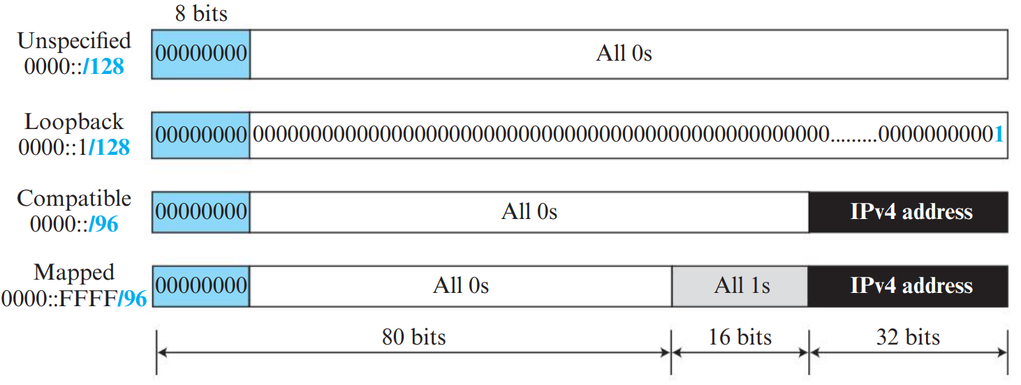
Special Addresses:
Unspecified Address: :: (all zeros).
Loopback Address: ::1.
IPv4-Mapped Address: ::ffff:192.168.1.1.
Figure 10.1: IPv6 40-Byte Fixed Base Header Format (Page 107)
2. IPv6 Fixed Base Header (40 Bytes Fixed)
Field Name
Bit Width
Technical Purpose
Version
4 bits
Value = 6 (binary 0110).
Traffic Class
8 bits
Replaces IPv4 ToS/DS; defines priority and congestion notification.
Flow Label
20 bits
Identifies packets belonging to the same real-time flow to enable fast hardware switching without deep packet inspection.
Payload Length
16 bits
Length of data and extension headers following the 40-byte base header.
Next Header
8 bits
Specifies the type of header immediately following (an extension header or transport protocol like TCP = 6, UDP = 17).
Hop Limit
8 bits
Replaces IPv4 TTL; decremented by 1 at each router.
Source Address
128 bits (16 bytes)
IPv6 address of the sending host.
Destination Address
128 bits (16 bytes)
IPv6 address of the receiving host.
⭐ Major Improvements in IPv6 Header over IPv4
Fixed Header Size: Fixed at 40 bytes; eliminates the HLEN field and speeds up hardware router processing.
No Header Checksum: Checksum removed; relying on link-layer CRC and transport-layer checksums eliminates router recalculation overhead!
No Mid-Path Router Fragmentation: Intermediate routers NEVER fragment IPv6 packets! If a packet exceeds link MTU, router drops it and sends ICMPv6 "Packet Too Big" so sender can use Path MTU Discovery.
📦 IPv6 Extension Headers Architecture
To keep the base header lean (40 bytes fixed), optional fields are chained together as Extension Headers linked via the Next Header field:
Extension Header
Next Header Code
Purpose & Functionality
Hop-by-Hop Options
0
Processed by every router along the path (e.g. jumbo payloads, router alert).
Routing Header
43
Specifies an explicit source-routing list of intermediate routers to visit.
Fragment Header
44
Contains fragmentation offset and ID when sender fragments a packet larger than path MTU.
Encapsulating Security Payload (ESP)
50
Provides data confidentiality, encryption, and authentication in IPSec.
Authentication Header (AH)
51
Provides data integrity, message authentication, and replay protection in IPSec.
Destination Options
60
Additional packet options inspected only by the final destination host.
3. Comprehensive Comparison: IPv4 vs. IPv6 (IPv4 vs IPv6)
Feature
IPv4
IPv6
Address Length
32 bits (4.3 billion addresses)
128 bits (\(3.4 \times 10^{38}\) addresses)
Base Header Size
Variable (20 to 60 bytes)
Fixed 40 bytes
Header Length (HLEN)
Present (4 bits)
No HLEN field (fixed 40 bytes)
Checksum
16-bit Header Checksum present (recalculated at every hop)
No checksum field (relies on L2/L4 checksums for speed)
Fragmentation
Performed by sending host AND intermediate routers
Performed exclusively by sender (Path MTU Discovery)
Packet Lifetime
Time to Live (TTL, in hops)
Hop Limit (in hops)
Protocol Field
8-bit Protocol field
Replaced by Next Header field
Security (IPSec)
Optional add-on
Mandatory native architectural support
4. Transition Strategies from IPv4 to IPv6 (Transition from IPv4 to IPv6)
Transition Strategy
Working Principle & Where Used
1. Dual Stack
Routers and hosts run both IPv4 and IPv6 protocol stacks simultaneously on the same machine. Can process both datagram types natively.
2. Tunneling
When two IPv6 networks must communicate across an intermediate IPv4-only network, the entire IPv6 datagram is encapsulated as payload inside an IPv4 packet!
3. Header Translation
Used when an IPv6-only host must communicate directly with an IPv4-only host. A NAT-PT gateway translates the IPv6 header into an IPv4 header and vice versa.
PART 11VERY HIGH PRIORITY • 5M / 9M ESSAY
Quality of Service (QoS) & Traffic Management
PDF Pages: 113 – 119
💡 What is Quality of Service (QoS)?
Traditional IP networks provide "best-effort" service. Real-time applications (VoIP, video conferencing, telemedicine) require performance guarantees regarding four key QoS metrics: Throughput (Bandwidth), Delay, Jitter (Delay Variation), and Packet Loss.
1. Traffic Shaping: Leaky Bucket vs. Token Bucket
Feature
Leaky Bucket Algorithm
Token Bucket Algorithm
Working Principle
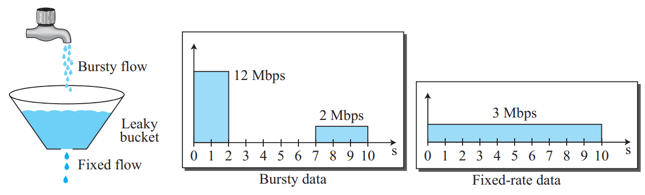
Packets enter a bucket of capacity \(C\) with a hole at the bottom. Water leaks out at a strictly constant uniform rate.
Tokens are generated at rate \(R\) and accumulate in a bucket of capacity \(B\). To transmit a packet, a token must be removed.
Bursty Output?
Never. Bursts are eliminated; output is completely smoothed to fixed rate.
Allows bounded bursts! If tokens are accumulated, a burst up to bucket capacity \(B\) can transmit at full wire speed.
Packet Dropping?
Drops packets if incoming burst overflows buffer capacity.
Drops only excess tokens; packets wait in queue if no tokens remain.
FIFO (First-In, First-Out): Simple queue; packets transmitted in exact arrival order. Zero differentiation.
Priority Queuing: High-priority traffic (e.g., VoIP) is transmitted first. Low-priority queues suffer from starvation during heavy load.
Fair Queuing & Weighted Fair Queuing (WFQ): Work-conserving scheduling where each flow gets a dedicated FIFO queue. In WFQ, each queue is assigned a weight \(w_i\) guaranteeing a proportional share of link bandwidth: \(\text{Bandwidth} = \frac{w_i}{\sum w_j} \times R\).
3. QoS Architectures: IntServ vs. DiffServ
Feature
Integrated Services (IntServ)
Differentiated Services (DiffServ)
Granularity
Per-flow QoS guarantees.
Per-class QoS aggregation.
Signaling Protocol
RSVP (Resource Reservation Protocol): reserves bandwidth along the entire end-to-end path.
No end-to-end signaling. Edge routers classify packets and mark the 6-bit DS field.
Router State
Stateful: core routers must maintain per-flow state.
Stateless core: core routers only implement Per-Hop Behaviors (PHB).
Scalability
Poor scalability in the Internet core (millions of flows).
High scalability; dominant Internet QoS architecture.
In Differentiated Services (DiffServ), packets are classified and marked at the network boundary using the 8-bit Differentiated Services (DS) field (former Type-of-Service / Traffic Class byte):
DSCP (6 bits): The first 6 bits define the Differentiated Services Code Point (DSCP), yielding up to 64 distinct service classes. The remaining 2 bits are reserved for Explicit Congestion Notification (ECN).
Per-Hop Behaviors (PHB): Internal routers inspect the DSCP to decide scheduling and drop precedence:
Expedited Forwarding (EF): Dedicated bandwidth with minimal delay, jitter, and loss (virtual leased line for VoIP).
Assured Forwarding (AF): 4 distinct classes and 3 levels of drop precedence within each class (e.g., gold, silver, bronze traffic).
Best Effort (BE): Default Internet traffic with no guarantees.
PART 12EXAM MASTERCLASS • NUMERICALS & QUESTION BANK
KTU Examination Masterclass & Solved Problems
📐 Master Numerical: Subnetting a Company Network
Problem: An organization is granted a block of addresses with the beginning address 190.100.0.0/16. The administrator wants to create 512 subnets. Find:
The subnet mask.
The number of addresses in each subnet.
The first and last address in Subnet 1.
Solution:
To create \(512 = 2^9\) subnets, we must borrow 9 bits from the host portion.
Number of addresses per subnet = \(2^{32 - 25} = 2^7 = \mathbf{128 \text{ addresses}}\) (126 usable hosts).
First subnet (Subnet 0): 190.100.0.0/25 to 190.100.0.127/25.
Subnet 1: 190.100.0.128/25 to 190.100.0.255/25.
KTU Module 2 Comprehensive Question Bank
Answer:
(i) File Transfer: TCP — Requires 100% reliable, error-free transmission. A single dropped bit corrupts a file.
(ii) Live Video Call: UDP — Requires low latency and real-time playback. TCP retransmission delays cause unacceptable freezing.
(iii) DNS Query: UDP — Requires fast, single-packet query-response with zero connection setup overhead.
Answer Blueprint:
Introduction (1 Mark): Define congestion and state that TCP controls congestion dynamically via the Congestion Window (\(cwnd\)).
Neat Graph Diagram (2 Marks): Draw \(cwnd\) versus Transmission Round (RTT), showing exponential growth up to \(ssthresh\), linear AIMD growth, timeout drop to 1, and 3-duplicate ACK Fast Recovery drop.
Slow Start (2 Marks): Starts at 1 MSS; doubles every RTT. Switches to Congestion Avoidance when \(cwnd \ge ssthresh\).
Congestion Avoidance (2 Marks): Additive increase by 1 MSS per RTT.