Interactive Study Environment • APJ Abdul Kalam Technological University
KTU 2024 SCHEME
9 CONTACT HOURS
THEORY MASTERCLASS
Module 4: Physical Layer & Network Management
Exhaustive masterclass covering Network Management (SNMP, SMI, MIB, FCAPS), ASN.1 & BER Encoding, Data & Signals, Theoretical Data Rate Limits (Nyquist & Shannon), Digital Transmission (Line Coding, Scrambling, PCM), Analog Transmission (ASK, FSK, PSK, QAM), Bandwidth Utilization (FDM, TDM, FHSS, DSSS), and Transmission Media (Twisted Pair, Coaxial, Fiber Optics, Wireless Bands).
54 Pages
Official PDF Notes Synthesized
89 Figures
High-Res Diagrams Embedded
12 Parts
Step-by-Step Learning Progression
100% Theory
Zero Omissions
💡 What is Network Management?
In a large enterprise network with thousands of heterogeneous routers, switches, and servers from different vendors, network administrators need a standardized way to monitor device health, configure parameters, detect link failures, and enforce security policies. SNMP is the universal framework for network management.
1. The Five Functional Areas of Network Management (FCAPS)
ISO defines five core functional areas of network management (remembered by the acronym FCAPS):
| Area | Acronym | Primary Purpose & Responsibility |
|---|
| Fault Management |
F |
Detects, isolates, logs, and corrects abnormal network component failures (e.g., link down, interface error). Automatically alerts administrators via trap alarms. |
| Configuration Management |
C |
Tracks and manages hardware/software settings, port configurations, IP addresses, firmware versions, and topology inventory across all managed devices. |
| Accounting Management |
A |
Monitors user and department resource consumption (bandwidth, connection time) for billing, capacity planning, and quota enforcement. |
| Performance Management |
P |
Monitors and analyzes network health metrics: throughput, packet drop rates, interface utilization, latency, and CPU load to prevent bottlenecks. |
| Security Management |
S |
Controls access to network devices, enforces firewall rules, manages encryption keys, authenticates administrators, and logs security breaches. |
2. The Triad of Network Management: SNMP, SMI & MIB
Network management in the Internet is divided into three distinct, cooperative standards:
| Component | Full Name | Role & Analogy |
|---|
| SMI |
Structure of Management Information |
The Language / Grammar: Defines rules for naming objects, defining object data types, and specifying how objects are encoded. |
| MIB |
Management Information Base |
The Database / Dictionary: The actual collection of managed objects and variables (e.g., packets in, packets out, interface status) stored inside each device. |
| SNMP |
Simple Network Management Protocol |
The Messenger / Protocol: Defines the message formats, request/response syntax, and communication procedures between managers and agents. |
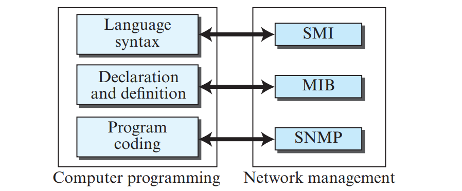
Figure 1.1: The Three Pillars of Network Management: SNMP, SMI, and MIB (Page 3)
1. SMI Object Identifier (OID) Hierarchy
SMI names all managed objects hierarchically using an Object Identifier (OID) Tree. Each node has a name and an integer number:
iso(1) . org(3) . dod(6) . internet(1) . mgmt(2) . mib-2(1) \(\implies\) 1.3.6.1.2.1
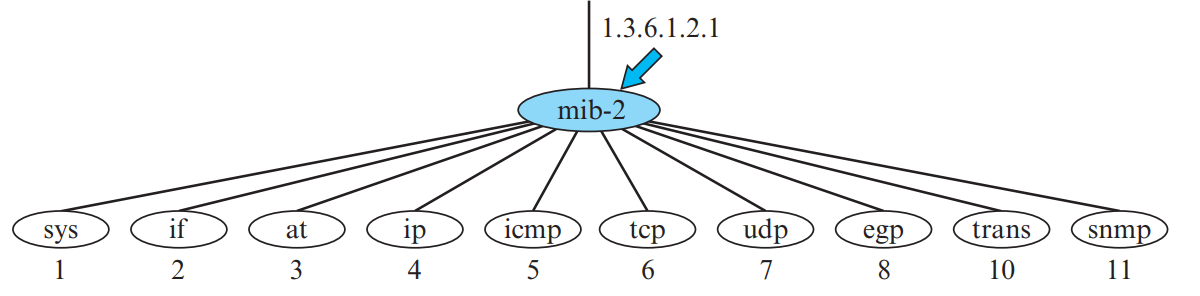
Figure 2.1: The Global SMI Object Identifier (OID) Tree Hierarchy (Page 7)
The 10 Core MIB-II Groups:
system (1): Device description, uptime, contact administrator.interfaces (2): Network interfaces, MTU, operational status, errors.at (3): Address translation (ARP table).ip (4): IP routing tables, forwarding stats, discarded packets.icmp (5): ICMP statistics (messages received, checksum errors).tcp (6): TCP connection parameters, active/passive opens, retransmission stats.udp (7): UDP statistics (e.g., udpInDatagrams = 1.3.6.1.2.1.7.1.0).egp (8), transmission (10), snmp (11).
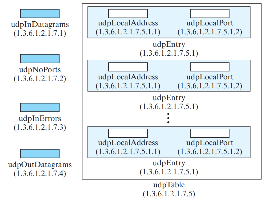
Figure 2.2: The MIB-II udp Group and 4-tuple Indexed udpTable (Page 8)
📋 SMI Data Types: Simple, Structured & Application-Wide
| Category | Type Name | Size | Behavior & Purpose |
|---|
| ASN.1 Simple Types | INTEGER | 4 bytes | Positive, zero, or negative integer values. |
OCTET STRING | Variable | Sequence of 0 to 65535 raw bytes (text strings, MAC addresses). |
OBJECT IDENTIFIER | Variable | Hierarchical sequence of numbers identifying an object in MIB tree. |
BITS | Variable | Bit string where each bit represents a specific flag or boolean status. |
| ASN.1 Structured | SEQUENCE | Variable | Ordered combination of fields (like a C struct or table row). |
SEQUENCE OF | Variable | Array of identical SEQUENCE objects (defines a complete table). |
| SMI Application-Wide | IPAddress | 4 bytes | 32-bit IPv4 address expressed as four octets. |
Counter32 | 4 bytes | Monotonically increasing counter (\(0\) to \(2^{32}-1\)); wraps back to zero when maxed. Used for cumulative traffic (packets/octets). |
Counter64 | 8 bytes | 64-bit high-capacity counter for high-speed Gigabit interfaces. |
Gauge32 | 4 bytes | Non-wrapping metric that can increase or decrease; upon reaching maximum (\(2^{32}-1\)), it latches at max until reset. Used for current temperature or active connections. |
TimeTicks | 4 bytes | Measures time elapsed in hundredths of a second (\(1/100\text{ s}\)) since device reboot or fixed epoch. |
🏛️ MIB-II Object Structure: Scalar vs. Tabular Objects
- Scalar Objects: Define a single distinct variable instance. In MIB-II notation, every scalar instance is addressed by appending
.0 to its object identifier (e.g. udpInDatagrams.0 has OID 1.3.6.1.2.1.7.1.0).
- Tabular Objects: Define multi-row database tables (like
udpTable with OID 1.3.6.1.2.1.7.5). Each row is an entry with multiple columnar variables, indexed by a primary key (e.g., local IP and port).
2. Basic Encoding Rules (BER) — TLV Format
SMI uses ISO Basic Encoding Rules (BER) to convert abstract data types into machine-independent byte streams for network transmission. Every data item is encoded using Tag, Length, Value (TLV):
| Field | Format | Description |
|---|
| Tag (T) | 1 byte | Identifies data type (e.g., 0x02 = INTEGER, 0x04 = OCTET STRING, 0x06 = OID, 0x30 = SEQUENCE). |
| Length (L) | 1 or more bytes | Specifies length of Value in bytes. |
| Value (V) | \(L\) bytes | The actual data value encoded in binary / two's complement. |
📐 High-Frequency KTU Numerical: BER TLV Encoding Examples
- Encode INTEGER 14:
Tag for INTEGER = 02 (hex).
Length = 1 byte \(\implies\) 01 (hex).
Value = 14 in hex is 0E.
\(\implies\) Encoded BER: 02 01 0E.
- Encode OCTET STRING "HI":
Tag for OCTET STRING = 04 (hex).
Length = 2 bytes \(\implies\) 02 (hex).
ASCII values: 'H' = 72 = 48 (hex), 'I' = 73 = 49 (hex).
\(\implies\) Encoded BER: 04 02 48 49.
📦 BER Tag Field Architecture & Concrete Encodings
In Basic Encoding Rules (BER), every object is encoded into Tag, Length, Value (TLV) octets. The Tag Byte consists of three subfields:
- Class (2 bits): Universal (
00), Application-wide (01), Context-specific (10), Private (11).
- Format (1 bit):
0 for Primitive data types; 1 for Constructed composite types (like SEQUENCE).
- Tag Number (5 bits): Identifies the type (INTEGER = 2 \(\implies\)
02, OCTET STRING = 4 \(\implies\) 04, NULL = 5 \(\implies\) 05, OID = 6 \(\implies\) 06, SEQUENCE = 16 \(\implies\) 30).
Real BER Encoding Examples (from Notes Page 7)
| Object / Type | Value | BER Hex Encoding | Detailed Byte Breakdown |
|---|
INTEGER | 14 | 02 04 00 00 00 0E | Tag = 02 (INTEGER), Length = 04 bytes, Value = 00 00 00 0E (hex for 14). (Or short form 02 01 0E). |
OCTET STRING | "HI" | 04 02 48 49 | Tag = 04 (OCTET STRING), Length = 02 bytes, Value = 48 49 ('H'=0x48, 'I'=0x49). |
OBJECT IDENTIFIER | 1.3.6.1 | 06 04 01 03 06 01 | Tag = 06 (OID), Length = 04, Sub-identifiers = 01 03 06 01. |
IPAddress | 131.21.14.8 | 40 04 83 15 0E 08 | Tag = 40 (Application class), Length = 04, Octets = 83 15 0E 08 (hex for 131, 21, 14, 8). |
1. SNMP Manager and Agent Architecture
Network management follows a client-server paradigm with specialized roles:
- SNMP Manager (Managing Entity): Central monitoring station/server running management applications. Polls agents, sends configuration requests, and receives alerts.
- SNMP Agent (Managed Entity): Software module running inside network devices (routers, switches, firewalls, printers). Collects local device statistics, answers manager queries, and fires trap alerts upon anomalies.
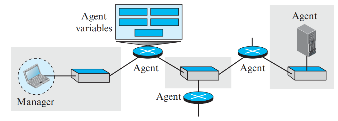
Figure 3.1: SNMP Manager-Agent Query and Trap Interaction (Page 2)
2. The Eight SNMP PDU Types (PDF Page 9)
| PDU Name | Direction | Purpose & Role |
|---|
| GetRequest | Manager → Agent | Retrieves the value of one or more specific MIB variables. |
| GetNextRequest | Manager → Agent | Retrieves the next lexicographical variable in the MIB tree (table traversal). |
| GetBulkRequest | Manager → Agent | Retrieves large blocks of tabular data in a single exchange (SNMPv2/v3). |
| SetRequest | Manager → Agent | Modifies or configures the value of a specific MIB variable on the agent. |
| Response | Agent → Manager | Returns the requested variable values or confirms a successful set action. |
| Trap | Agent → Manager | Unsolicited asynchronous alarm reporting an unexpected event (SNMPv1). |
| InformRequest | Manager → Manager | Alert message sent from one NMS to another NMS, requiring an acknowledgment. |
| SNMPv2-Trap | Agent → Manager | Modernized unsolicited notification reporting exceptional events (SNMPv2/v3). |
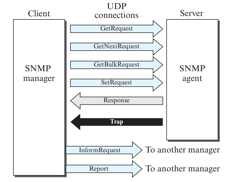
Figure 3.2: Direction of Flow for the 8 SNMP PDU Types (Page 9)
3. Transport Protocol & Port Numbers
SNMP operates over UDP because of its low overhead and ability to function even when network links are heavily congested:
- UDP Port 161 (Agent Listening Port): The Agent listens passively on port 161. Managers send
GetRequest, GetNextRequest, GetBulkRequest, and SetRequest to port 161.
- UDP Port 162 (Manager Trap Port): The Manager listens passively on port 162. Agents send unsolicited
Trap and InformRequest messages to port 162.
💡 What is ASN.1?
ASN.1 is a standard formal notation used to define data structures and types independent of machine architecture, word size, or operating systems. SMI uses a subset of ASN.1 to define MIB objects.
1. ASN.1 Lexical Conventions & Syntax Rules
- Assignment Symbol:
::= means "is defined as".
- Comments: Begin with double hyphen
-- and end at end of line or another --.
- Type Names: Must start with an UPPERCASE letter (e.g.,
INTEGER, StudentAccount).
- Variable / Value Names: Must start with a LOWERCASE letter (e.g.,
johnNewton, studentAge).
2. ASN.1 Data Types
| Category | ASN.1 Type | Description & Example Definition |
|---|
| Simple Types | BOOLEAN | Contains values TRUE or FALSE. |
INTEGER | Positive or negative whole numbers; can have named values or range constraints. |
BIT STRING | Ordered sequence of zero or more bits (e.g., '0110'B or '4F'H). |
OCTET STRING | Ordered sequence of zero or more 8-bit bytes (text strings, binary). |
| Structured Types | SEQUENCE | An ordered list of heterogeneous fields (equivalent to a struct in C). |
SEQUENCE OF | An ordered list of homogeneous elements (equivalent to an array in C). |
⭐ High-Frequency KTU Question: Identifying Errors in ASN.1 Declarations
Sample Problem: Identify errors in the following declarations and correct them:
studentAge INTEGER = 21
Error: Used = instead of assignment operator ::=.
Correct: studentAge INTEGER ::= 21
classSize NumberOfStudents ::= 50 (where NumberOfStudents ::= INTEGER (1..40))
Error: Value 50 violates the subrange constraint (1..40).
Correct: Value must be between 1 and 40 (e.g., classSize NumberOfStudents ::= 35).
EmployeeName ::= octet string
Error: Built-in types must be written in ALL-CAPS: OCTET STRING.
Correct: EmployeeName ::= OCTET STRING
📑 ASN.1 Structured Types & Subtyping Rules
- CHOICE: Defines a list of mutually exclusive alternatives where only one data type can be selected (e.g.
Weekend ::= CHOICE { saturday NULL, sunday NULL }).
- Subtyping Constraints: Restricts the allowable value range or size of built-in data types:
- Range Constraints: Limits numeric values using
.. (e.g. NumberOfStudents ::= INTEGER (15..40), Grade ::= REAL (1.0..5.0)).
- Size Constraints: Limits length of octet strings (e.g.
ShortName ::= OCTET STRING (SIZE (1..10))).
💡 Role of the Physical Layer
The Physical Layer is the only layer where data is converted into physical energy (voltages, light pulses, or electromagnetic waves) and transmitted across a physical medium.
1. Data & Signals: Analog vs. Digital, Time vs. Frequency Domain
Data can be analog (continuous, like human voice) or digital (discrete states, like computer data). To be transmitted across a physical medium, data must be converted into electromagnetic signals:
- Analog Signals vs. Digital Signals:
- Analog Signals: Have infinitely many levels of intensity over a continuous period. Represented mathematically as sinusoidal waves: \(s(t) = A \sin(2\pi f t + \phi)\).
- Digital Signals: Have a limited number of discrete defined values (typically binary: 0 and 1). Maintain constant voltage levels during bit intervals with instantaneous transitions.
- Periodic vs. Aperiodic Signals:
- Periodic: Completes a cycle within a measurable period \(T\) and repeats identical patterns over time (\(f = 1/T\)).
- Aperiodic (Non-periodic): Changes without exhibiting any repeating pattern over time. Real-world digital network data is inherently aperiodic.
- Time Domain vs. Frequency Domain (Fourier Analysis):
- Time Domain Plot: Shows signal amplitude changes with respect to time.
- Frequency Domain Plot: Shows the amplitude and phase of each frequency component (spectral lines). According to Fourier analysis, any composite signal is a combination of multiple simple sine waves.
🌊 Sine Wave Parameters
A simple analog periodic signal is represented by a sine wave: \(s(t) = A \sin(2\pi f t + \phi)\), defined by three parameters:
- Peak Amplitude (\(A\)): The absolute maximum value or highest intensity of the signal, measured in volts, amperes, or watts.
- Frequency (\(f\)) & Period (\(T\)): Frequency is the number of complete cycles per second (\(\text{Hz}\)); Period is the time required to complete 1 cycle (\(T = 1/f\)).
- Phase (\(\phi\)): The position of the waveform relative to time zero, measured in degrees or radians.
- Wavelength (\(\lambda\)): The distance a signal propagates in one period: \(\lambda = v \times T = v / f\) (where \(v\) is propagation speed).
2. Transmission Impairments & Decibel Calculations
Signals experience three primary types of transmission impairments as they travel across physical media:
| Impairment | Cause & Mechanism | Effect on Signal | Mitigation Technique |
|---|
| Attenuation | Resistance of medium dissipates electrical/optical energy as heat over distance. | Loss of signal amplitude and strength. | Amplifiers (analog) or Repeaters (digital). Formula: \(\text{dB} = 10 \log_{10}(P_2/P_1)\) (10 log power ratio formula). |
| Distortion | Different frequency components travel at different speeds (delay distortion) in composite signals. | Changes composite signal shape and phase relationships. | Equalizers at receiver. |
| Noise | External unwanted electrical signals corrupting the transmitted waveform. | Flipping bits, causing data errors. | Shielding, differential signaling, higher SNR. |
Categories of Noise in Communications
- Thermal Noise (Johnson/Nyquist noise): Random motion of free electrons in conductors; unavoidable and uniformly distributed across all frequencies (white noise).
- Induced Noise: Electromagnetic interference (EMI) radiated from motors, generators, power lines, and fluorescent ballasts acting as transmitting antennas.
- Crosstalk: Unwanted capacitive or inductive coupling between adjacent wire pairs (e.g. hearing another conversation on an analog phone line).
- Impulse Noise: High-voltage, short-duration spikes from lightning or power surges; the primary cause of burst errors in digital communications.
1. Nyquist Bit Rate (For Noiseless Channels)
Formulated by Harry Nyquist in 1928 for an ideal, noiseless channel of bandwidth \(B\) using \(L\) discrete signal levels:
\[\text{Bit Rate} = 2B \log_2(L) \quad \text{bps}\]
Standard formula: Bit Rate = 2B log2(L) bps (where \(B\) is bandwidth in Hertz, and \(L\) is the number of signal levels).
2. Shannon Capacity (For Noisy Channels)
Formulated by Claude Shannon in 1944. Defines the ultimate theoretical upper bound on channel capacity (\(C\)) in the presence of thermal white noise:
\[C = B \log_2(1 + \text{SNR}) \quad \text{bps}\]
Standard formula: Capacity C = B log2(1 + SNR) bps (theoretical upper limit in a noisy channel).
Crucial Insight: Notice that the Shannon formula has no signal level \(L\) term! No matter how many signal levels an engineer designs, the data rate can never exceed the Shannon capacity without increasing bandwidth or reducing noise.
📐 High-Frequency KTU Numerical Problem: Combining Shannon & Nyquist
Problem: A channel has a bandwidth of 1 MHz and a signal-to-noise ratio (\(\text{SNR}\)) of 63. Calculate:
- The theoretical maximum channel capacity (Shannon capacity).
- The number of signal levels \(L\) required to achieve a bit rate of 4 Mbps using the Nyquist formula.
Solution:
- Shannon Capacity:
\[C = B \log_2(1 + \text{SNR}) = 1 \times 10^6 \times \log_2(1 + 63) = 10^6 \times \log_2(64)\]
Since \(64 = 2^6\), \(\log_2(64) = 6\).
\[C = 10^6 \times 6 = \mathbf{6 \text{ Mbps}}\]
(The absolute physical ceiling of this channel is 6 Mbps).
- Signal Levels for 4 Mbps:
We want \(\text{Bit Rate} = 4\text{ Mbps}\). By Nyquist formula:
\[4 \times 10^6 = 2 \times B \times \log_2(L) = 2 \times (1 \times 10^6) \times \log_2(L)\]
\[4 = 2 \log_2(L) \implies \log_2(L) = 2 \implies L = 2^2 = \mathbf{4 \text{ signal levels.}}\]
💡 What is Line Coding?
Line coding converts a sequence of binary digital bits (1s and 0s) into a digital voltage signal suitable for transmission over a wire. Desirable characteristics: self-synchronization (clock recovery), no DC component, noise immunity, and bandwidth efficiency.
1. Five Major Line Coding Schemes & Waveform Characteristics
Line coding converts a sequence of digital bits into a digital signal waveform. Schemes are broadly classified into:
- Unipolar (NRZ - Non-Return to Zero): Uses only one non-zero voltage level (e.g., \(+V\) for bit 1, \(0\text{ V}\) for bit 0). Suffers from massive DC component (average signal voltage is non-zero) and lack of self-synchronization during long runs of 0s or 1s.
- Polar Schemes: Use voltages on both sides of zero (\(+V\) and \(-V\)):
- NRZ-L (NRZ-Level): Voltage level depends strictly on bit value (e.g. \(+V\) for 0, \(-V\) for 1).
- NRZ-I (NRZ-Invert): Inversion or transition at the beginning of the bit interval denotes bit 1; no transition denotes bit 0.
- RZ (Return-to-Zero): Signal transitions to zero volts halfway through every bit interval, providing guaranteed clock synchronization at the expense of doubling bandwidth.
- Manchester: Transition in the middle of every bit interval: low-to-high represents bit 0, high-to-low represents bit 1. Combines clock and data; used in 10 Mbps Standard Ethernet.
- Differential Manchester: Transition at the middle of the interval provides synchronization; transition at the beginning represents 0, absence of transition at the beginning represents 1.
- Bipolar (AMI - Alternate Mark Inversion): Three voltage levels (\(+V, 0\text{ V}, -V\)). Bit 0 is represented by \(0\text{ V}\); bit 1 is represented by alternating positive and negative pulses. Completely eliminates DC component, but long strings of zeros cause clock synchronization loss.
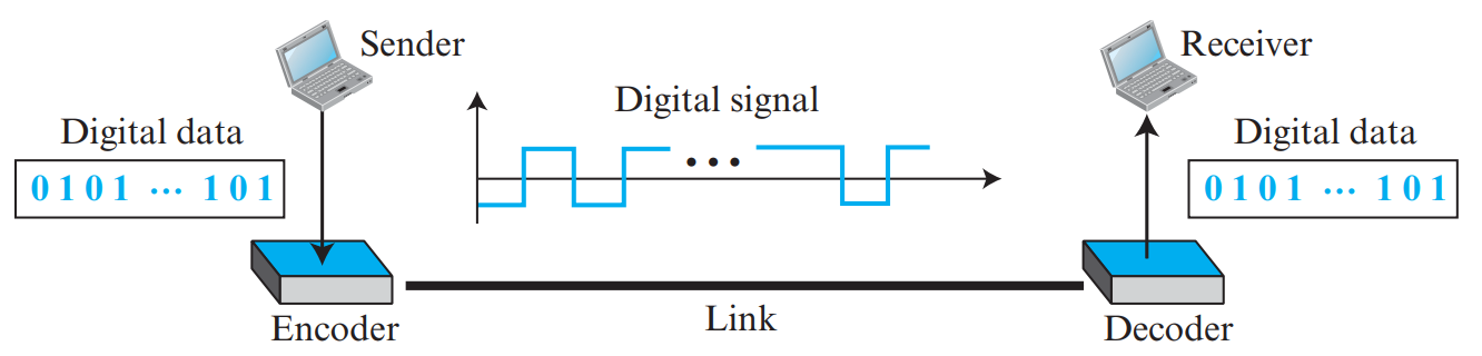
Figure 7.1: Line Coding Waveforms: NRZ-L, NRZ-I, RZ, Manchester, and Differential Manchester (Page 27)
| Scheme | Encoding Rule for '0' | Encoding Rule for '1' | Self-Sync & DC Component |
|---|
| NRZ-L (Level) |
Positive voltage level (\(+V\)). |
Negative voltage level (\(-V\)). |
No self-sync during long runs of 0s or 1s. Has strong DC component. |
| NRZ-I (Invert) |
No transition at start of bit interval. |
Invert (transition) at start of bit interval. |
Self-syncs on 1s, but loses sync during long runs of 0s. |
| RZ (Return-to-Zero) |
Negative level returns to zero at midpoint. |
Positive level returns to zero at midpoint. |
Good sync, but uses 3 voltage levels and doubles bandwidth! |
| Manchester |
Transition from HIGH to LOW at midpoint. |
Transition from LOW to HIGH at midpoint. |
Perfect self-synchronization! (Used in 10 Mbps Ethernet). Zero DC component. Doubles bandwidth. |
| Differential Manchester |
Transition at the beginning of the bit interval. |
No transition at the beginning of bit interval. (Always transitions at midpoint). |
Excellent noise immunity and perfect self-sync. (Used in Token Ring). |
| Bipolar AMI |
Zero voltage (0 V). |
Alternating positive and negative voltages (\(+V, -V, +V...\)). |
Zero DC component. Long runs of 0s lose synchronization. |
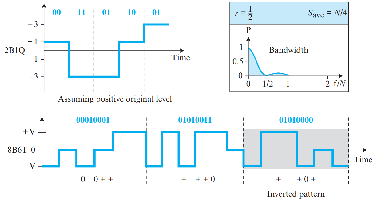
Figure 7.2: Bipolar AMI: Zero Level for '0', Alternating Polarities for '1' (Page 29)
⚡ Line Coding Characteristics: Baseline Wandering & Baud Rate
- Baseline Wandering: In decoding incoming digital signals, the receiver calculates a running average of received signal power called the baseline. Long sequences of consecutive 0s or 1s shift this baseline voltage (baseline wandering), causing the receiver to misinterpret signal thresholds and drop bits.
- DC Component: When voltage levels remain on one side of zero for extended periods, low frequencies around zero (DC component) are created. Media with transformers or capacitors cannot pass DC components.
- Baud Rate (Signal Rate \(S\)) vs. Bit Rate (\(N\)):
- Bit Rate (\(N\)): Number of data bits transmitted per second (\(\text{bps}\)).
- Baud Rate / Signal Rate (\(S\)): Number of signal element transitions (symbols) per second (\(\text{baud}\)).
- Relationship: \(S_{\text{ave}} = c \times N \times \frac{1}{r}\) (where \(c\) is the case factor, typically \(1/2\), and \(r\) is data bits per signal element).
2. Scrambling: B8ZS and HDB3
Used with Bipolar AMI to eliminate long runs of zeros without increasing the transmission bit rate (unlike Manchester):
- B8ZS (Bipolar with 8-Zero Substitution - North America): Replaces eight consecutive zeros (
00000000) with the deliberate bipolar violation pattern: 000VB0VB (where \(V\) is violation of AMI polarity, and \(B\) conforms to AMI).
- HDB3 (High-Density Bipolar 3 - Europe): Replaces four consecutive zeros (
0000) with either 000V (if odd number of non-zero pulses since last substitution) or B00V (if even count).
Figure 7.3: B8ZS Substitution Pattern: 000VB0VB (Page 31)
💡 Why Digitize Analog Signals?
Human voice and music are continuous analog waveforms. Converting analog data to digital bits allows transmission over noise-immune digital networks, encryption, compression, and computer processing.
1. The Three Steps of Pulse Code Modulation (PCM)
-
Step 1: Sampling:
The continuous analog signal is sampled at periodic intervals of \(T_s\).
Nyquist Sampling Theorem: The sampling frequency \(f_s\) must be at least twice the highest frequency component (\(f_{\text{max}}\)) of the analog signal:
\[f_s \ge 2 \times f_{\text{max}}\]
-
Step 2: Quantization:
The continuous sampled voltage amplitudes are rounded to the nearest discrete quantization level. If \(n_b\) bits are used per sample, the number of quantization levels is:
\[L = 2^{n_b}\]
The difference between the actual sample and the rounded value is the Quantization Error (\(\Delta\)).
-
Step 3: Encoding:
Each quantized level is translated into an \(n_b\)-bit binary code word.
Digital Bit Rate Formula:
\[\text{Bit Rate} = f_s \times n_b = 2 \times f_{\text{max}} \times n_b \quad \text{bps}\]
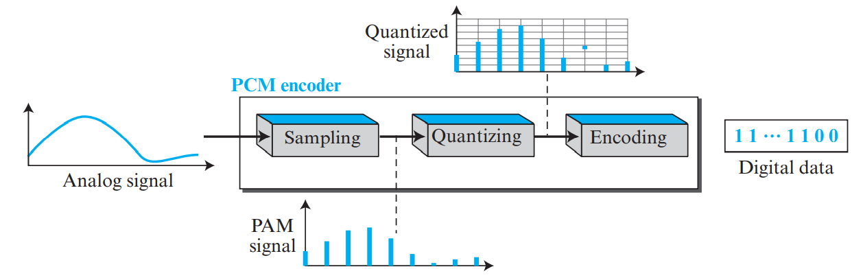
Figure 8.1: Sampling: Ideal, Natural, and Flat-Top (Page 33)

Figure 8.2: Quantization Levels & Binary Encoding (Page 34)
📐 High-Frequency KTU Numerical Problem: PCM Telephone Voice Digitization
Problem: A human voice signal has a bandwidth of 4 kHz. It is digitized using PCM with 8 bits per sample (\(n_b = 8\)). Find:
- The Nyquist sampling rate.
- The resulting bit rate.
- The theoretical SNR in decibels (\(\text{SNR}_{\text{dB}}\)).
Solution:
- \(f_{\text{max}} = 4\text{ kHz}\).
- Sampling rate \(f_s = 2 \times 4\text{ kHz} = \mathbf{8000 \text{ samples/second}}\).
- Bit Rate \(= f_s \times n_b = 8000 \times 8 = \mathbf{64 \text{ kbps}}\) (the universal digital telephone DS0 voice channel!).
- \(\text{SNR}_{\text{dB}} = 6.02 \times n_b + 1.76 = 6.02(8) + 1.76 = \mathbf{49.92 \text{ dB}}\).
🎙️ Non-Linear Quantization: Companding (A-law & μ-law)
In human speech, soft sounds occur far more frequently than loud sounds. Linear uniform quantization produces large relative quantization errors for soft whisper signals. To optimize fidelity:
- Companding (Compressing + Expanding): The analog input signal is non-linearly compressed at the transmitter (amplifying weak signals more than strong signals), uniformly quantized and encoded, and expanded at the receiver using the inverse logarithmic transfer curve.
- Standard Companding Laws:
- μ-law (mu-law): Standard in North America and Japan (\(\mu = 255\)):
\[y = \frac{\ln(1 + \mu |x|)}{\ln(1 + \mu)} \cdot \operatorname{sgn}(x)\]
- A-law: Standard in Europe and international ITU-T telecommunications (\(A = 87.6\)):
\[y = \frac{1 + \ln(A |x|)}{1 + \ln A} \cdot \operatorname{sgn}(x) \quad \text{for } \frac{1}{A} \le |x| \le 1\]
2. Delta Modulation (DM)
Instead of sending full 8-bit values for each sample, DM sends only 1 bit per sample indicating whether the signal is increasing (1) or decreasing (0). Uses a simple staircase approximation.
- Slope Overload Distortion: Occurs when the analog signal rises faster than the staircase can climb.
- Granular Noise: Occurs when the analog signal is flat, causing the staircase to oscillate around it.
💡 Why Carrier Modulation?
Bandpass channels (radio airwaves, cable TV, long-distance telephone lines) cannot transmit baseband square waves. Digital bits must modulate the amplitude, frequency, or phase of a high-frequency sinusoidal carrier wave.
1. Carrier Modulation & Digital-to-Analog Schemes
In analog transmission, digital data modulates a high-frequency sinusoidal Carrier Signal: \(c(t) = A_c \cos(2\pi f_c t + \phi)\), altering one or more of its characteristics:
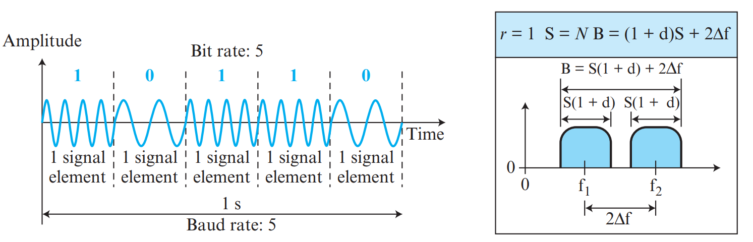
Figure 9.1: Waveforms for ASK, FSK, and PSK Aligned with Digital Data (Page 37)
| Technique | What Changes | What Remains Constant | Bandwidth Formula |
|---|
| ASK (Amplitude Shift Keying) |
Carrier amplitude changes (bit 1 = high amplitude, bit 0 = zero amplitude in OOK). |
Frequency and Phase. |
\(B = (1 + d) \times S\) |
| FSK (Frequency Shift Keying) |
Carrier frequency changes (\(f_1\) for 1, \(f_2\) for 0). |
Amplitude and Phase. |
\(B = (1 + d) \times S + 2\Delta f\) |
| PSK (Phase Shift Keying) |
Carrier phase shifts (BPSK: 0° for bit 1, 180° for bit 0). |
Amplitude and Frequency. |
\(B = (1 + d) \times S\) |
| QAM (Quadrature Amplitude Modulation) |
Both amplitude AND phase vary simultaneously. |
Frequency. |
Same as PSK, but carries \(\log_2(L)\) bits per baud! |
2. Constellation Diagrams & QAM
A constellation diagram plots signal states on a 2D polar plane: the horizontal \(X\)-axis represents the in-phase carrier, and the vertical \(Y\)-axis represents the quadrature carrier. A 16-QAM constellation has 16 points, carrying \(n = \log_2(16) = \mathbf{4 \text{ bits per signal element}}\)!
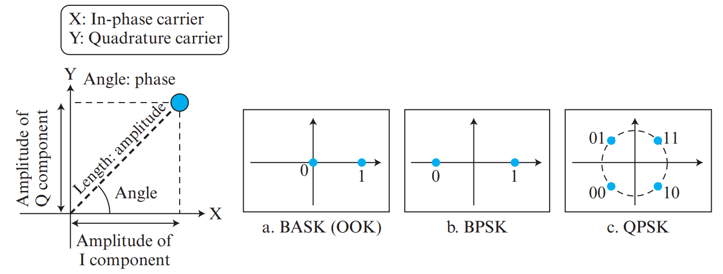
Figure 9.2: Constellation Diagrams for BPSK, QPSK, 8-QAM, and 16-QAM (Page 38)
💡 What is Bandwidth Utilization?
A physical transmission line often has far more bandwidth than an individual communication flow requires. Multiplexing allows multiple low-rate channels to share a single high-capacity medium. Spread Spectrum expands a signal's bandwidth over a wide band to provide military-grade anti-jamming, privacy, and noise immunity.
1. Multiplexing Techniques: FDM, WDM & TDM
- FDM (Frequency-Division Multiplexing): Analog technique. The available physical bandwidth is divided into non-overlapping frequency bands, separated by unallocated guard bands to prevent interference (e.g., Radio and Cable TV).
- WDM (Wavelength-Division Multiplexing): Optical counterpart of FDM. Multiple light wavelengths (colors) propagate through a single optical fiber.
- TDM (Time-Division Multiplexing): Digital technique. High-speed channel time is divided into recurrent time slots; each user is assigned a specific time slot in each frame.
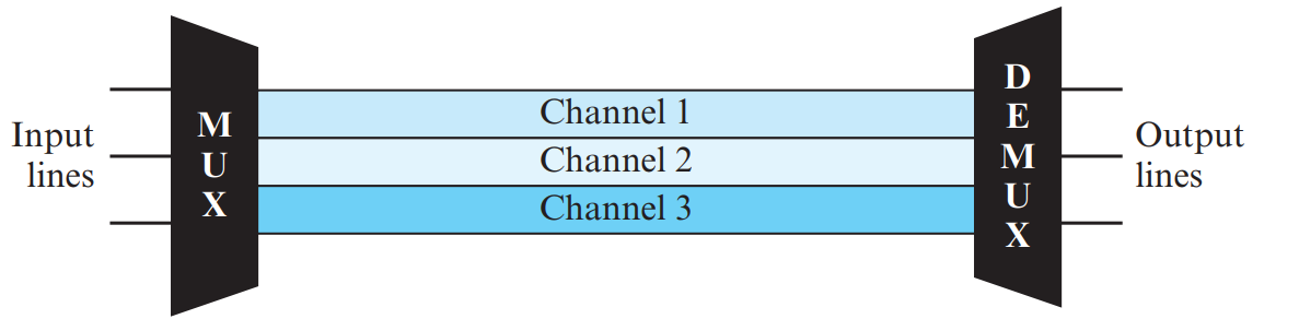
Figure 10.1: Frequency-Division Multiplexing (FDM) with Guard Bands (Page 43)
Synchronous TDM vs. Statistical TDM (PDF Page 45 – 46)
| Comparison Parameter | Synchronous TDM | Statistical (Asynchronous) TDM |
|---|
| Slot Allocation |
Pre-allocated fixed slots to every input line in a round-robin cycle. |
Slots allocated dynamically on-demand only to input lines that currently have data to send. |
| Channel Efficiency |
Low. If an input line has no data, its allocated time slot goes empty and is wasted! |
High. Zero empty slots; bandwidth is fully packed. |
| Addressing Overhead |
No addressing needed; slot position implicitly identifies the sender. |
Every slot must carry an address tag identifying destination/source. |
| Buffer Requirements |
Minimal buffering required. |
Requires memory buffers at multiplexer during peak bursts. |
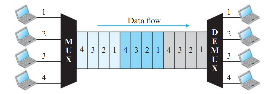
Figure 10.2: Synchronous TDM (Empty Wasted Slots) vs Statistical TDM (Dynamic Slots) (Page 45)
2. Spread Spectrum: FHSS vs. DSSS
📡 Spread Spectrum Mechanics: PN Code & Chipping Rate
Spread spectrum techniques intentionally expand the transmission bandwidth to achieve security, anti-jamming, and multi-user access:
- Frequency Hopping Spread Spectrum (FHSS): The carrier frequency switches rapidly among \(M\) different channels guided by a pseudo-random sequence. The time spent at each frequency is the dwell time.
- Direct Sequence Spread Spectrum (DSSS): Each original data bit is multiplied by an \(N\)-bit PN code (Pseudorandom Noise code) chip sequence.
- Chipping Rate: The rate at which the PN code chips are generated (\(f_{\text{chip}} \gg f_{\text{data}}\)). The bandwidth expansion factor is given by the ratio of the chipping rate to the data bit rate.
| Feature | Frequency Hopping Spread Spectrum (FHSS) | Direct Sequence Spread Spectrum (DSSS) |
|---|
| Working Principle |
Signal modulates a carrier that hops rapidly between different frequencies according to a pseudo-random sequence. |
Each original data bit is multiplied by an \(n\)-bit high-rate pseudo-random Barker chip sequence. |
| Bandwidth Expansion |
Frequency band is divided into \(M\) hopping channels. |
Signal bandwidth is expanded by a factor of \(n\) (\(\text{Chip Rate} = n \times N\)). |
| Applications |
Bluetooth (1600 hops/second), military communications. |
Wi-Fi (802.11b), GPS, CDMA cellular networks. |
| Benefits |
Highly resistant to narrowband frequency jamming and eavesdropping. |
Immune to multi-path fading, allows simultaneous shared access (CDMA). |
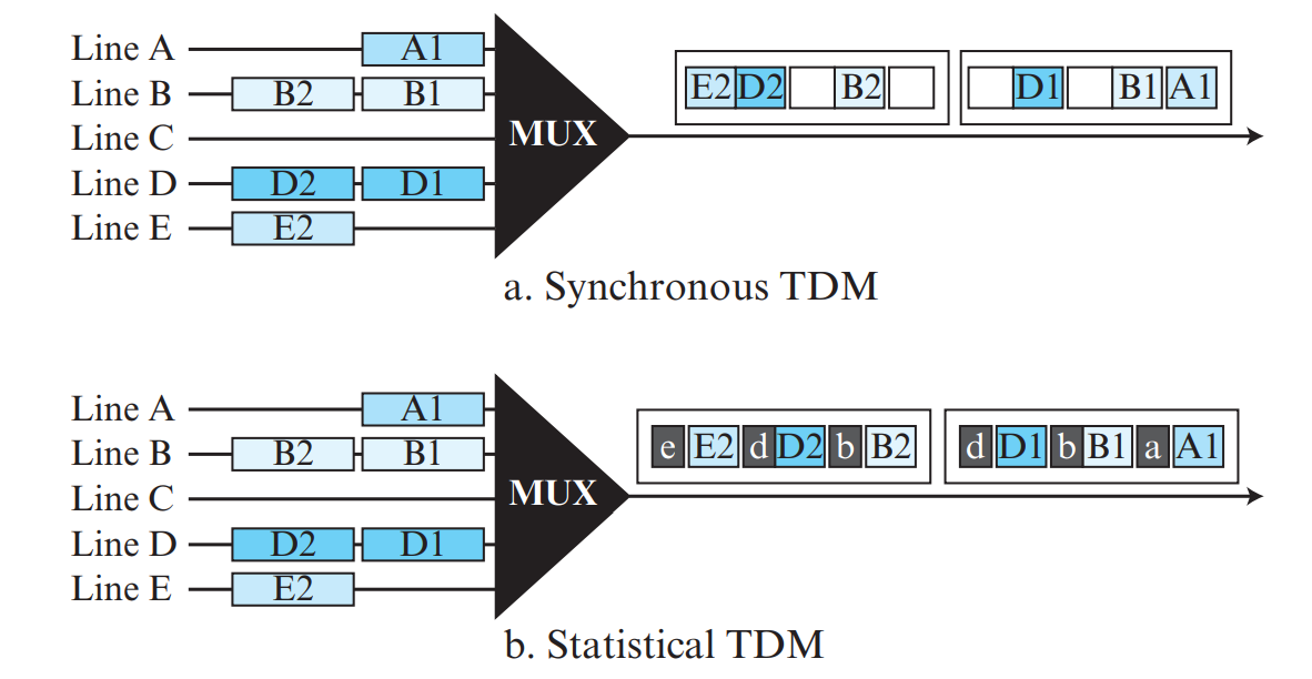
Figure 10.3: Spread Spectrum Principles: Frequency Hopping (FHSS) and Direct Sequence (DSSS) (Page 47)
1. Guided Transmission Media (Guided media: Cables)
Guided media provide a physical conduit from one device to another:
| Medium Type | Physical Construction | Bandwidth & Attenuation | Immunity & Use Case |
|---|
| Twisted-Pair (UTP / STP) | Two insulated copper conductors twisted in a helical spiral to cancel electromagnetic induction and crosstalk. | 10 Mbps – 10 Gbps depending on Category (Cat 5e, Cat 6, Cat 6a). | Low cost; standard for Ethernet LAN drops (RJ-45 connectors). |
| Coaxial Cable | Central solid copper core surrounded by dielectric insulator, braided foil/metal shield, and outer jacket. | Higher bandwidth than twisted-pair; lower attenuation. | Cable television (CATV), broadband internet, legacy 10Base5/10Base2. |
| Fiber-Optic Cable | Glass or plastic core surrounded by lower-density cladding and protective buffer jacket. | Terabits/sec; extremely low attenuation over tens of kilometers. | Immune to EMI, noise, and wiretapping; backbone Internet trunks. |
Optical Physics: Refraction, Critical Angle & Total Internal Reflection
- Refraction & Snell's Law: When light passes from a medium of higher refractive index \(n_1\) (core) to a lower refractive index \(n_2\) (cladding), the ray bends away from the normal:
\[n_1 \sin \theta_1 = n_2 \sin \theta_2\]
- Critical Angle (\(\theta_c\)): The angle of incidence where the refracted ray travels along the boundary surface (\(\theta_2 = 90^\circ\)):
\[\theta_c = \arcsin\left(\frac{n_2}{n_1}\right)\]
- Total Internal Reflection: When the angle of incidence exceeds the critical angle (\(\theta_1 > \theta_c\)), light cannot penetrate the cladding and is 100% reflected back into the core, guiding the beam through the fiber.
- Propagation Modes:
- Multimode Step-Index: Multiple light rays bounce at sharp angles down the core; high modal dispersion limits distance.
- Multimode Graded-Index: Core density varies parabolically from center to edge, bending rays smoothly and equalizing travel times.
- Single-Mode: Extremely narrow core (\(\approx 8\text{ – }10\ \mu\text{m}\)) permitting only a single axial light beam (laser source); virtually zero modal dispersion for ultra-long hauls.
2. Unguided Transmission Media (Unguided media: Wireless)
Unguided media transport electromagnetic waves without using a physical conductor. Wireless propagation occurs through the atmosphere or free space across three primary frequency bands:
| Wireless Band | Frequency Range | Propagation Mode | Characteristics & Applications |
|---|
| Radio Waves | 3 kHz – 1 GHz |
1. Ground wave: < 2 MHz follows Earth curvature.
2. Sky wave: 2 – 30 MHz reflects off the ionosphere.
3. Line-of-sight: > 30 MHz straight line between antennas.
| Omnidirectional (sends in all directions); penetrates walls easily. Used in AM/FM radio, television, paging. |
| Microwaves | 1 GHz – 300 GHz | Line-of-sight propagation | Unidirectional (focused beams via parabolic dish or horn antennas); cannot penetrate solid walls well. Used in cellular, satellite, and Wi-Fi. |
| Infrared Waves | 300 GHz – 400 THz | Line-of-sight propagation | High frequency; cannot penetrate walls, preventing interference between adjacent rooms; no government frequency license required. Used in TV remote controls and short-range wireless peripherals. |
📐 Master Waveform Question: Draw NRZ-L, NRZ-I and Manchester (KTU 6 Marks)
Problem: Draw the line coding waveforms for the bit sequence 1 0 1 1 0 0 1 for:
- NRZ-L (Non-Return-to-Zero, Level)
- NRZ-I (Non-Return-to-Zero, Invert on 1)
- Manchester
Waveform Guide:
- Bit Sequence:
1 0 1 1 0 0 1
- 1. NRZ-L: Bit 1 = Negative Voltage (\(-V\)); Bit 0 = Positive Voltage (\(+V\)).
Voltages: \(-V, +V, -V, -V, +V, +V, -V\).
- 2. NRZ-I: Transition at start of bit for '1'; No transition for '0'.
Assume initial state before bit 1 is negative.
• Bit 1: Inverts \(\rightarrow\) High.
• Bit 0: No invert \(\rightarrow\) stays High.
• Bit 1: Inverts \(\rightarrow\) Low.
• Bit 1: Inverts \(\rightarrow\) High.
• Bit 0: No invert \(\rightarrow\) stays High.
• Bit 0: No invert \(\rightarrow\) stays High.
• Bit 1: Inverts \(\rightarrow\) Low.
- 3. Manchester: Midpoint transition: '0' = High-to-Low (\(\downarrow\)); '1' = Low-to-High (\(\uparrow\)).
Midpoint transitions: \(\uparrow, \downarrow, \uparrow, \uparrow, \downarrow, \downarrow, \uparrow\).
KTU Module 4 Comprehensive Question Bank
Answer:
- SMI (Structure of Management Information): Defines the grammar and rules for naming objects, defining object data types, and specifying how objects are encoded using ASN.1.
- MIB (Management Information Base): The database holding the collection of managed objects, tables, and variables residing inside each managed network device.
- SNMP (Simple Network Management Protocol): The application-layer communication protocol that defines the message formats (PDUs) exchanged between managers and agents over UDP ports 161 and 162.
Answer Blueprint:
- Introduction (1 Mark): Define PCM as the standard method for converting an analog waveform into digital bits.
- Step 1: Sampling & Nyquist Theorem (3 Marks): Draw analog curve with vertical sample pulses. State that sampling frequency must satisfy \(f_s \ge 2 f_{\text{max}}\) to prevent aliasing.
- Step 2: Quantization & Quantization Error (2.5 Marks): Explain dividing amplitude into \(L = 2^{n_b}\) discrete levels. Define quantization error \(\Delta\) and give \(\text{SNR}_{\text{dB}} = 6.02 n_b + 1.76\text{ dB}\).
- Step 3: Encoding & Bit Rate (2.5 Marks): Show converting levels into binary codewords. Give bit rate formula \(\text{Bit Rate} = f_s \times n_b\) and telephone voice 64 kbps example.
⚡ Module 4 Last-Minute Memory Mnemonics
- Network Management Areas: FCAPS → Fault, Configuration, Accounting, Performance, Security.
- SNMP UDP Ports: Agent listens on 161; Manager Trap listens on 162.
- Shannon Capacity: \(C = B \log_2(1 + \text{SNR})\).
- Nyquist Rate: \(\text{Bit Rate} = 2 B \log_2 L\).
- PCM Telephone Bit Rate: \(8000 \text{ samples/s} \times 8 \text{ bits/sample} = \mathbf{64 \text{ kbps}}\).
- Half-Power Loss: \(10 \log_{10}(0.5) = \mathbf{-3 \text{ dB}}\).